Scaling Rectified Flow Transformers for High-Resolution Image Synthesis

Section 1: a new architecture for rectified flow that allows it to scale for problems that are not class-conditioned generation

• using ImageNet and CC12M rather than CIFAR-10 and CelebA 64x64 like used in the original rectified flow paper

Section 2 Deriving training objective for ODE vector field prediction

coming up with a unifying formula for the training objective of ODE-based flow models (like rectified flow) and diffusion models. I swear I’ve seen like a bajillion of these, and it seems the general idea is that they’re all predicting some kind of noise or equivalently, velocity

Based on a schedule for flowing from x_0 in p_0 to p_1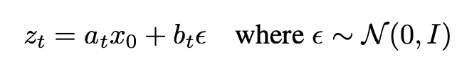

You can derive the marginal vector field u_t(z), which is what you’re trying to get your vector field network output to predict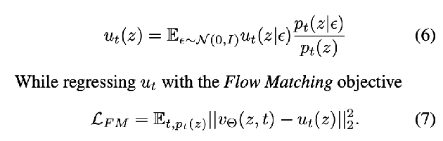

But the marginalization makes it intractable, so, it’s actually equivalent to use the conditional flow matching objective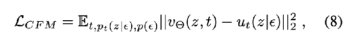

plug back in the conditional vector field expression u_t(z|epsilon), reparameterize using the SNR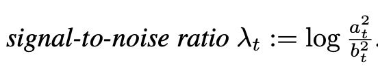

and make the network output predict epsilon instead of v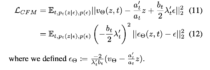

Finally, introducing a weighting term by time leaves the optimum the same but changes some of the optimization dynamics, but allows us to unify different perspectives.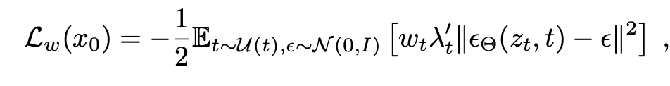

where L_CFM corresponds to a particular choice of w_t

Section 3: How different flow variants fall under this formalism, with different a_t and b_t defining the forward path, different network output, results in a setting for w_t in general: changing the forward path changes which noise scales (what SNR level?) the model learns most strongly based on the resulting w_t

Rectified Flow: 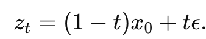, so a_t = 1-t, b_t = t

• network output parameterizes velocity, not noise trained using L_CFM ⇔ w_t = t/(1-t)

EDM: 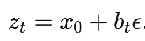(adding different noise levels on top of the data), a_t = 1, 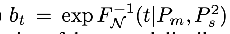, network output is the noise

Cosine: 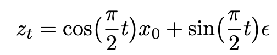, variance preserving: a_t^2 + b_t^2 = 1 network output is the noise

Section 3.1: the velocity is a lot easier to learn at t=0 and t=1 than in the middle (since you’re calculating E[v = eps - x_0], but at t=0 you know x_0, and at t=1 you know eps . Want to reweight the RF weighting term to favor the middle, using a distribution π(t) that’s not the uniform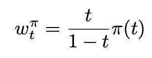

They try three different densities:

• logit-normal (literally run a normal through a logit so it ends up in (0, 1)
• mode sampling with heavy tails (parameter s controls where mass goes)
• Keep straight rectified flow but take the speed of going along the path from CosMap

Section 4 Architecture

get coarse grained global view of the text input through c_vec, from concatenating CLIP-L/14 and CLIP-G/14 encodings. This gets fed into the layer modulation (the Ada-LN-Zero weights)

c_ctxt is the fine grained sequence representation of the text, from concatenating CLIP-L/14 and T5 XXL encodings. This is fed into the attention blocks together with the image patch sequence (but with a different set of weights, so that only the attention part is combined)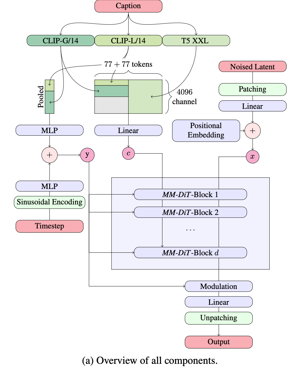

• red are the different inputs (and the output). Going one by one through how these are processed:
• noised latent: patched + embedded, positional embeddings added to the sequence, and just fed into the attention blocks as a sequence.
• caption: used for both the modulation and the sequence attention like we mentioned above.
  • the big rectangle is showing that in order to concatenate the 77 token length sequence from T5 XXL, with each token being 4096 dimensional, with the 77 token length sequence from CLIP-G/14 and CLIP-L/14, which are lower dimensional. You need to pad the remaining dimensions with the gray 0’s block
• timestep: time is encoded using sinusoidal encoding, added together with the CLIP c_vec to get the modulation input y

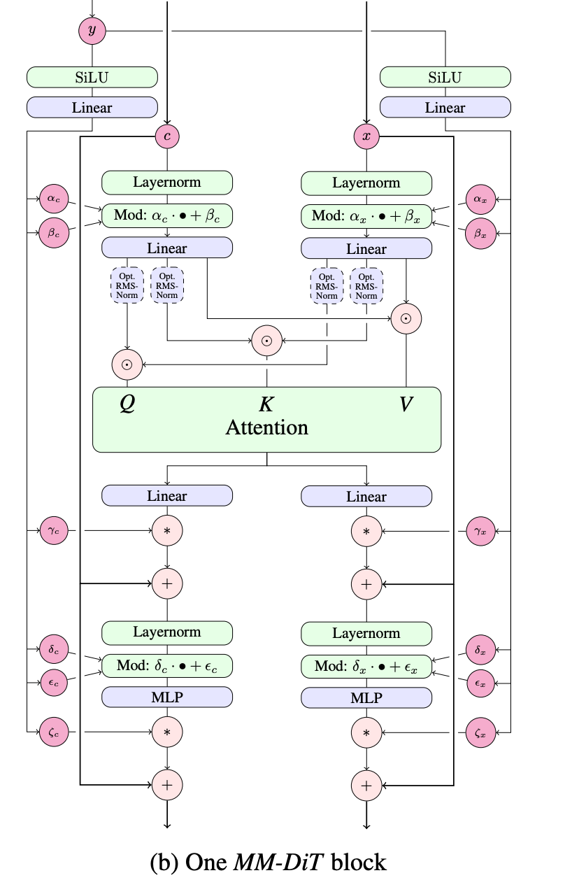dual streams to process the text and the noised image by attention

• layernorm is the standard layernorm in transformer blocks, is what allows us to do this modulation using y
• the circle . means concatenation, i.e. the two streams for text and image are concatenated only for the attention layers and otherwise have different weights and modulation
• notice the residual connection everywhere
• optional rmsnorm on the queries and keys for large models in order to keep the softmax from being dominated by one query key pair. Cheaper than doing another layernorm (and turns out to be sufficient)

MM-DiT (this arch) beats DiT, Cross attention DiT (not bidirectional like MM-DiT, the text sequence tokens don’t look at the image tokens), UViT

Ablate the inclusion of T5 as well (Or rather during inference time, I think, because they train using dropout, so they can choose to not include it during inference time)

Section 5 Experiments

comparing different training methods (holding the architecture and optimization) constant on COCO-2014 validation split Metrics

• CLIP-FID (normal FID uses inception v3). CLIP-FID is more accurate for text to image generation

find that rectified flow with the logit normal works pretty well across the board

Tricks for scaling up:

• use a latent with a larger channel dimension d for the VAE (intuition: it’s harder to predict more channels d)
• use 50% actual captions, 50% synthetic captions (the human captions are often sparse and leave stuff out about the background)
• filter out bad data
• pre-compute the text and image embeddings once for the entire dataset
• mixed precision training causes instability on higher resolution image fine tuning (pretraining is on lower resolution usually), for those, add in the RMSNorm and it learns the RMSNorm properly even if you didn’t do include it during pretraining time

Handling images with different resolutions.

• Positional encoding: They batch images with similar resolutions. They create a master grid that is the max height and width of any image in the batch. Then they use for each image the positional encodings of a center cropped version of this master grid.
• When you have higher resolution, it takes more noise to get down to the same level of information in the image. This means that when you are sampling noise levels / time steps t to train at, the level of information left at a given time step is different for different resolutions.
  • so you probably don’t want to use the uniform for everything. You sample from one of the distributions (like uniform, or logit normal), and then you transform the t using the shift function and use that t for your training step
    • this shift function is mathematically motivated by just 1/sqrt(n) scaling of variance, but in practice they fit it empirically
  • more discussion about this noise / time shift in the Flux 2 technical reports summary

You can apparently fine tune a lora on the Diffusion model further using DPO (appendix C)

Results: Beyond qualitative comparisons, also used the GenEval and human preference on the Parti-prompts benchmark

• Sota on GenEval (Benchmark tests for specific things showing up in the generated images).
• Scaling laws: Validation loss smoothly goes down as you increase the depth of the model and increase the number of training FLOPs
• Lower validation loss corresponds with better final metrics.
• The T5 encoder is more important for making sure the typography is consistent, and less so for other properties of the image.