Flow Straight and Fast: Learning to Generate and Transfer Data with Rectified Flow

Motivation: Diffusion models are very slow at inference time because they have to go through many steps. If we could just straighten out the path from source to target distribution, we could only take one step

Intuitions and goodness of Rectified Flow

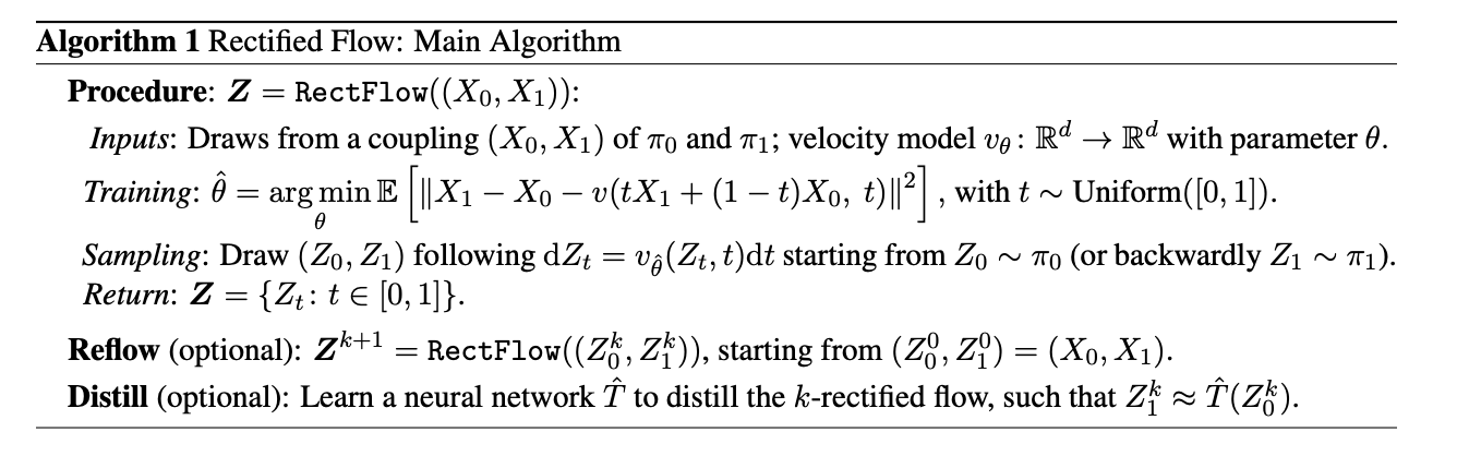
Try to learn a transport function from X_0 to X_1 by predicting the velocity X_1 - X_0 at any point in time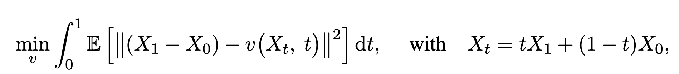

X_1 is not known at inference time, so, training v to predict it

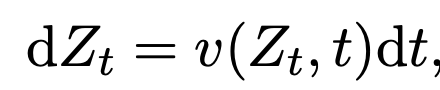
Can get forward and backward processes out of this ODE.
Equally favored because training is time-symmetric.
straight means straight with a constant speed, i.e. in a path from Z_0 to Z_1, v(Z_t, t) is constant

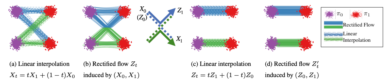
The linear interpolation paths can cross, but paths from an ODE can’t cross at the same time and place (because it has a unique solution, i.e. v(Z_t, t) can’t take on two different values at the same point)

Good property 1 of rectified flow: Rectify converts an arbitrary coupling (X_0, X_1) to a causal, deterministic coupling (Z_0, Z_1) with lower transport costs

Good property / corollary 2: If you keep applying rectify to this new coupling (Z_0, Z_1) -> (Z_0’, Z_1’), you get straighter and straighter paths with lower and lower transportation costs.
Straighter paths mean less euler sampling error, fewer steps needed.

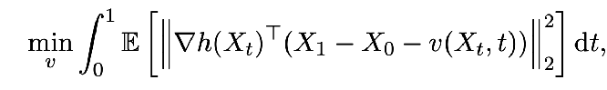
If the neural network was able to minimize the error perfectly, it would learn 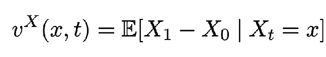What are some properties of the coupling (Z_0, Z_1) resulting from this velocity field?

marginal of Z_t = the marginal of X_t at every t (in particular, is a valid coupling of pi_0 and pi_1)
- Because for a fixed x and t, same expected total mass (flux) moving through that point under Z_t (following v^T) and X_t (following the linear interpolation) are the same
- It doesn’t optimize for any one particular transport cost.
- Intuitively, this holds because Rectify rewires crossing paths
- tradeoff: More reflow steps cause higher error.

Distilling: Learn to approximate the final coupling in one step.

Approximating v^X: Use deep neural networks for high dimension and Nadaraya-Watson for low dim

Comparison to diffusion

In general, can approximate non-linear interpolations too, but lose the straightening guarantees.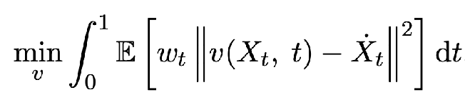

their choice of beta_t makes the paths non straight
their choice of alpha_t makes the speed non-uniform

Everyone in the past try to extract ODEs out of SDEs, but Rectified Flow just learns the ODE directly. I like this phrasing from Related Works “However, because PF-ODEs and DDIM were derived as the side product of learning the mathematically more involved diffusion/SDE models, their theories and algorithm forms were made unnecessarily restrictive and complicated.”

Section 3 Theoretical Analysis

3.1 rigorously proving that the marginals are equal. tbh don’t understand the math but whatever

recall the intuition for this was same flux at each point and time

3.2 convex costs go down when you apply rectify. Used jensen’s for the math (I think the idea is that at each (x, t), you only have one direction v^X(x, t) instead of many X_1 - X_0’s, and then averaging with Jensen’s makes it go down or something.
Recall the intuition was that non-intersecting paths have lower distance cost

3.3 Straightness means that at each point and time, There is already only one path X_0 X_1 passing through it, So rectify doesn’t do anything to the coupling.
The O(1/k) rate comes from this telescoping sum where they show that the straightnesses add up to E[ X_1^2 - X_0^2 ] which is finite

3.4 Straightness is necessary but not sufficient for an optimal transport for a given function c. Except in 1D, where it’s sufficient because it implies monotonicity (larger X_0 implying larger X_1)

3.5 They show that the training objective of VE, VP, sub-VP SDEs matches the Rectified Flow objective. Not sure what’s going on here either

ODEs > SDEs

numerically better, easily time reversible, couplings being deterministic makes them useful latent spaces for outputs, same expressivity for marginals,
ODEs better for modeling smooth manifold data, SDEs probably better for modeling highly noisy data (like financial markets)

Experiments

Toy examples seem to mostly be for figures, bunch of gaussian mixtures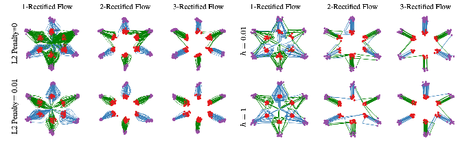

figure 7, l2 penalty helps straighten flows for neural networks (left)

Unconditional image generation on CIFAR-10

used a Unet for their v predictions
metrics: Frechet Inception Distance (FID) and Inception Score (IS) for quality, recall score for diversity
The table 1 results lowkey look kinda noisy, idk what the clear takeaways about what methods are better is
even in Figure 8, seems like 2-reflow is between 1 and 3 reflow in behavior, which is kinda weird. But I guess reflow better in small step regime (because straighter paths) and worse in large # steps regime (because accumulating error) makes sense
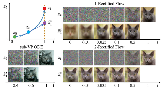
Figure 10 is actually pretty good, shows straightening in the sense that with 2-rectified flow, even from early time, if you predict the full output that you’re heading towards, it stays pretty constant
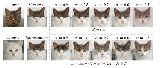
Figure 12 is a cool application of the reverse process. You stitch two images together, run the reverse process which should give you some low probability Z_0, then you push it towards a more high probability region, and then you rerun the forward process

Image to Image Translation — transferring the style from one image to another image while maintaining the main subject

X_0, X_1 are both meaningful distributions but don’t want to just faithfully reconstruct X_1, want to keep the main subject of X_0 train a classifier, focus on the interpolation getting from one class to another

all analysis was qualitative which makes this kinda sus

Domain Adaptation Experiment

Apparently there’s datasets DomainNet and OfficeHome with a bunch of categories of the same image taken from different settings, so trying to see if they can alleviate domain shift issues in classification by transferring to a training domain first using rectified flow