Same Task, Different Circuits: Disentangling Modality-Specific Mechanisms in VLMs
modality specific circuits
Trying to understand why tasks are easier in language than in vision.
Actually, a super good figure 1 summarizing their contributions 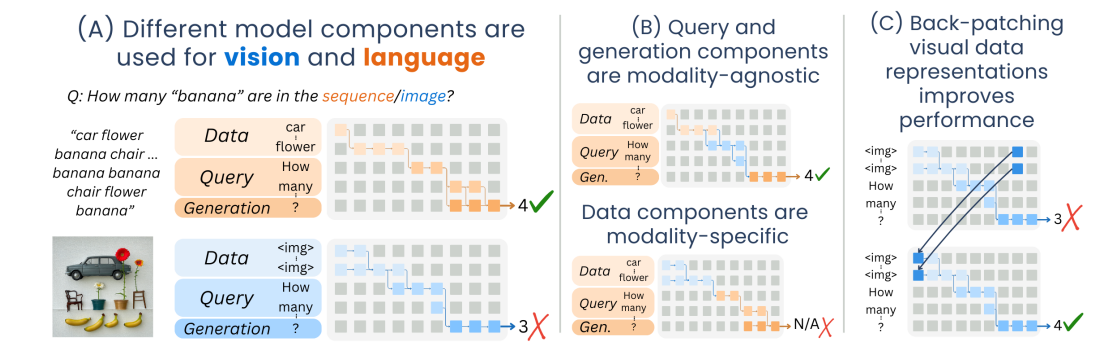
- This is straight up the entirety of the introduction as well.
Section 2 circuit discovery and evaluation
Circuit nodes are attention heads or individual MLP neurons. I think they’re not claiming to find edges in this one.
Discovery: Ideally, you would take your original and counterfactual prompts and see patching at which nodes causes the most change in the logits of the answers. But there are too many components, so instead they use attribution patching with integrated gradients. 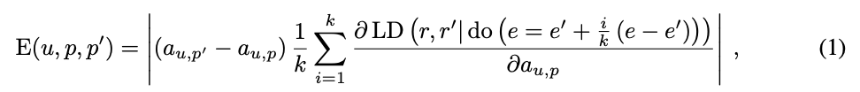
- LD is the logit difference.
-
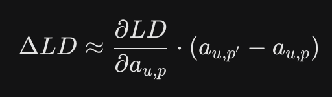
- This is the normal first-order approximation for the effect on the larger difference of the activation patch.
- But this is a little inaccurate. To do better, we have a k-piece discretization of the interpolation from the original prompt embedding e to the new prompt embedding e’
Faithfulness evaluation. A little different from previous ways of measuring faithfulness based on Mueller et al. 2025 instead of Wing et al. 2022 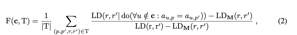
- For each prompt p in the task, randomly pick a counterfactual p’. Patch over all the non-circuit nodes from p’. (first numerator term). Normalize by the logit difference is when you patch all model components and when you patch no model components.
- Counterfactual ablation instead of mean ablation because the mean might not be typical of any of the individual activations (“off-manifold”)
- This normalization technique seems to be generally applied: subtract a random / baseline, and divide by what would happen for the oracle/whole, to keep you in [0, 1]
Figure 4: at about 7% of components for textual task circuits and 15% of components for visual tasks, achieves 80% faithfulness on the task 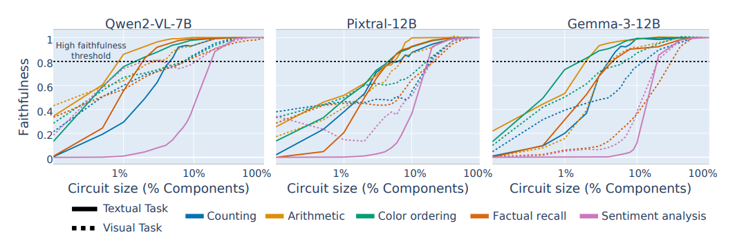
Section 3 Experimental setup
Figure 2: Their tasks in textual and visual form. 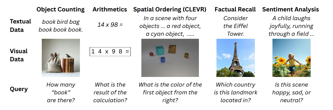
- Answers need to be one word, and prompts need to be aligned to a positional template, for Circuit Discovery to work well (guess they don’t use PEAP)
Qwen2-7B-VL-Instruct, Pixtral-12B, Gemma-3-12B-it
- Adapter Architecture: Pre-trained image encoder -> Visual token embeddings -> Adapter layer -> Language embedding space -> Concatenated with text and passed through language decoder
Section 4. Analyzing the circuits
Motivated by Kaduri et al 2024 and the different patching effects (averaged over all components) for the data query and generation prompt positions (Figure 3), split circuits into data, query, and generation. 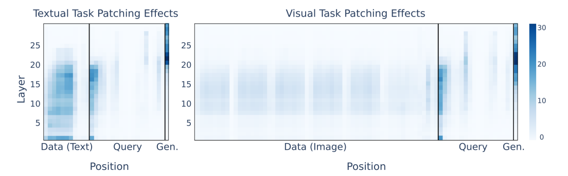
Figure 5: There is very little overlap in the data processing part between the circuits in different modalities, with more overlap in the generation part 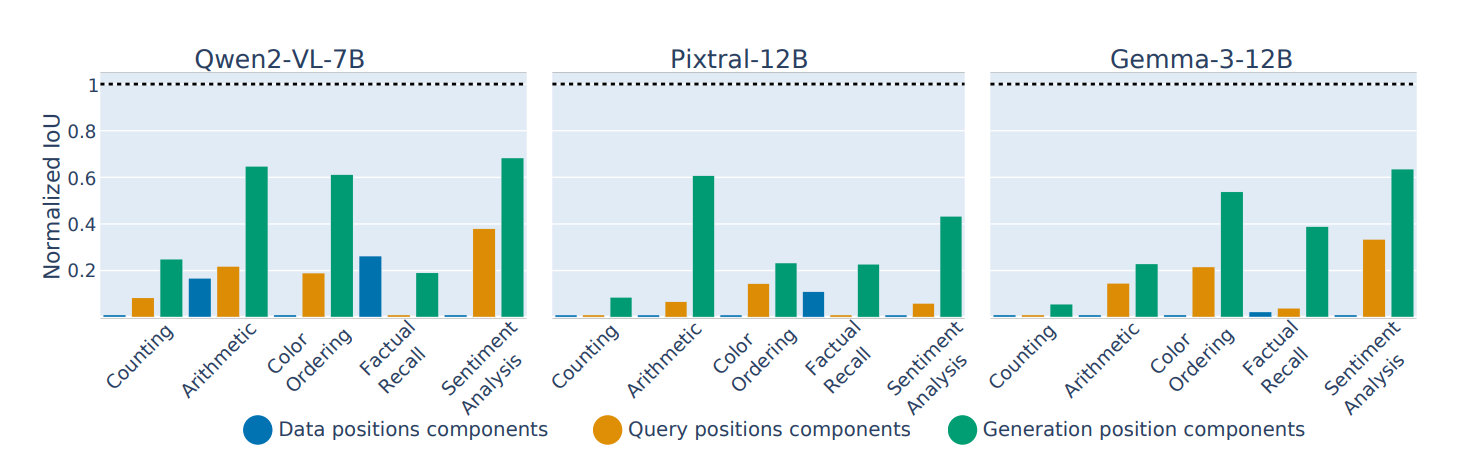
- Generally want to calculate the IoU between the components in the circuits for text versus for vision (These circuits are discovered independently on separate data sets)
- You can align the positions within the query and generation components, but for the data processing components, they just dropped the token position from the label of the node.
- Calculate IoUs separately for MLP and attention heads and average them together, since many more MLP neurons than attention heads
- Normalize by the random chance overlap between random circuits to account for the bias of a larger circuit size. (nIoU vs IoU)
Figure 6: When you patch over the query or generation components of one modality into the circuit for the other modality. Faithfulness still is retained. But not for the data processing components. So functionally, the circuits are similar, even though structurally, from Figure 5, they aren’t. 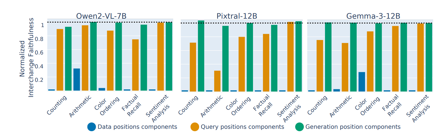
- Patching means literally just taking the circuit components, replacing the components for query or generation, and then doing the same counterfactual ablation as before.
- Normalization in this case is patching in a random sub-circuit as a baseline, and the original circuit as the oracle
Section 5. Back patching image representations to improve performance
this part is kind of sus to me since it’s not really related to the circuit they discovered. It’s only barely motivated by the fact that the data processing circuit seems to be very different between the modalities.
Figure 7: Averaged over each visual patch token, They compute the maximum cosine similarity to any text token (in a separate generation) for each layer. This cosine similarity goes up as you go later into layers, Suggesting that later layer image representations are more aligned with the text 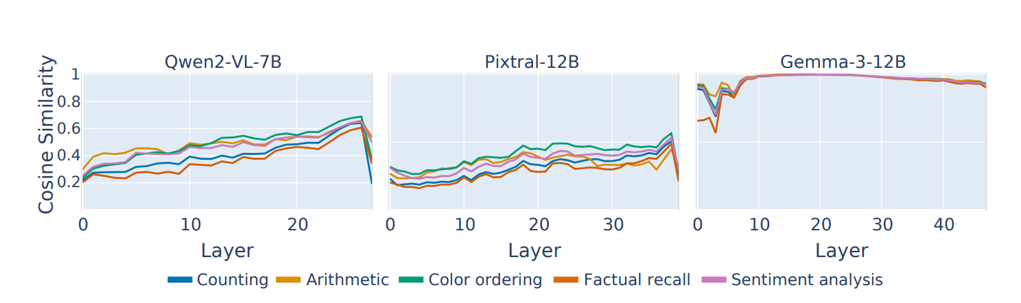
So what they do instead, is do one full generation with the images. They capture later representations for the image tokens, and then they patch that into earlier layers of a new generation (This doesn’t leak task info because of Autoregressiveness, and the image coming first in the prompt).
Table 1: This improves results by a little bit.
They confirm that it’s not due to just extra computation, by also doing this patching for text, and it improves results much less for text.