Section 2: Randomness

1111111… isn’t random because LLN says that random strings should be 50% 0’s and 50% 1’s 1010101… isn’t random because it’s predictable

Martin-Lof randomness / Kolmogorov complexity: random if no short Turing machine can distinguish from true random

cryptographic randomness (pseudorandom number generator): no polynomial time alg can distinguish from true random

• good enough in most settings because if you’re doing a polynomial time computation, then if using a PRG instead of a true RG made a difference, that would be a poly time alg to distinguish from true random

Section 3: Defining epiplexity

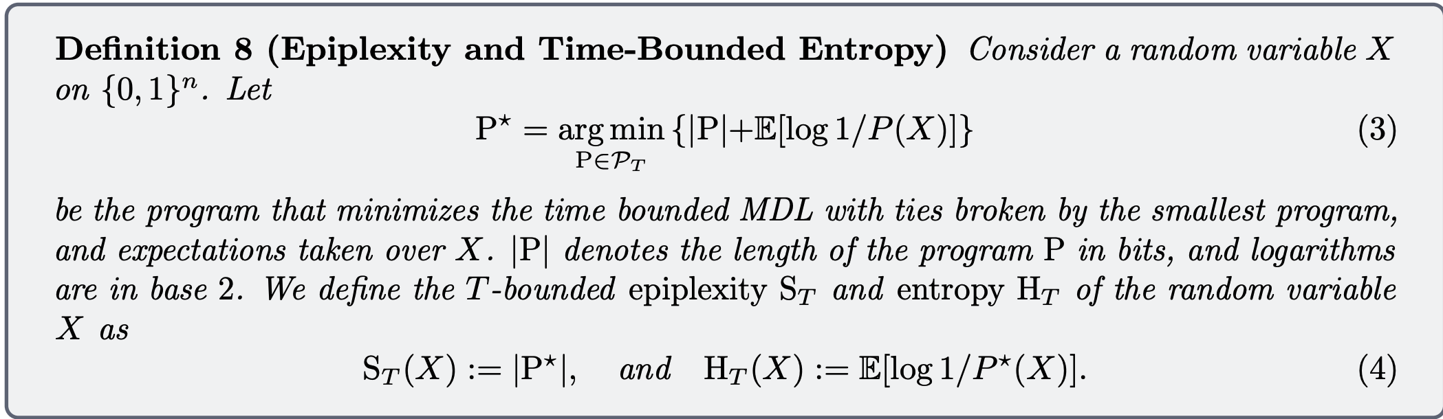
• MDL = minimum description length = size of the program + entropy left using the program (think Occam’s razor, simplest program that explains it sufficiently)
• Epiplexity is just the length of the program part. The rest of it is the “time-bounded entropy”
• the time-bounded is from only allowing programs within a certain time complexity

Examples:

• Uniform and Pseudo random number generators are low epiplexity high time-bounded entropy, since you can describe their minimum programs (the generators) pretty easily. Kolmogorov gives a somewhat higher complexity to PRGs; Gemini is telling me that this is mainly because epiplexity is defined on a random variable, while Kolmogorov complexity is defined on a fixed string, so you can hardcode the seed for the latter but not for the former. Hence, epiplexity concludes that there’s no poly-time learnable structure, while Kolmogorov complexity says that there is.

Section 4: Two methods of calculating Epiplexity on real datasets

Info theoretical setup: encoder has access to the test set $X$ and possibly teacher model checkpoints, decoder starts with just the base student model. They’re trying to minimize epiplexity (program length) + remaining entropy of the entire test set $X$. Theoretically, the test set $X$ is the entire dataset of interest that we’re trying to measure the epiplexity of, but in practice we use a held-out test split and rescale it to the size of the entire dataset.

• epiplexity: we’re going to approximate programs as trained neural nets. Program length is roughly the number of bits / code that you need to transmit to a student, and the hard thing is how to measure the minimum number of bits that you need. There are two ways to do this:
  • prequential coding: you’re handing over the actual data over the channel. The decoder maintains their own synchronized copy of the model as the encoder is training it, and on step $i$, the encoder takes the next piece of data $Z$, uses the current model (that the decoder has) to calculate how many bits it is, and then sends that over the channel, and repeats for all the data.
    • this is too pessimistic, since it includes the remaining entropy of the data under the final trained model, so you adjust by subtracting the number of bits that you’d still have to send to encode the data if you had the trained model from the start. Note that this doesn’t tell you how to actually achieve the subtracted number of bits through a code, it’s non-constructive
    • this corresponds to area under the training loss curve (see below)
  • requential coding: instead of passing over real data, we can pass over synthetic data generated by the teacher checkpoints the encoder has access to.
    • This somehow takes less bits to encode, and furthermore is an explicit construction of the number of bits passed that we’re claiming.
    • This corresponds to the area between the loss curves
• remaining entropy: after you have the trained model, you can just run a forward pass of the model on the test data $X$ to get the remaining entropy

And note that we’re trying to minimize this at an outer loop to find the MDL. They do this minimization just by trying a bunch of hyperparameters and taking the one with the lowest score.

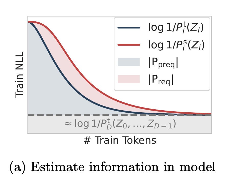
• prequential = area under the training loss curve
• requential = area between the teacher and student loss curves

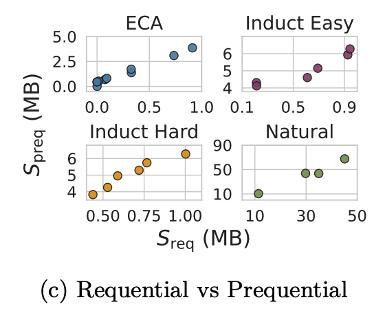
• in practice, prequential and requential seem to agree. Prequential is cheaper since it just requires the one training run

Section 5. Epiplexity fixes 3 paradoxes of normal info theory

The common theme is just that restricting the computation of the observer explains the new information created in all three of these phenomena

5.1: post-processing doesn’t give new information

This is only true if you assume unlimited computation time. In that sense, run the deterministic AlphaZero RL doesn’t generate new information you didn’t have before. But it does if you don’t have the time to redo that computation

Notably, theoretically you only produce new information even with compute-constrained entropy if the inverse is not efficient. “some useful guidance for synthetic data: if we want to produce interesting information, we should make sure the functions we use do not have simple and efficiently computable inverses”

• inverses means for instance deriving the original from the generated
• do I believe this? I feel like this means most data augmentations are useless

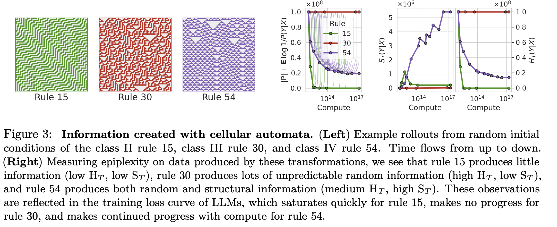
• three types of cellular automata synthetic data generation. Only rule 54 is high epiplexity

5.2 order should matter

Shannon entropy treats H(X, Y) and H(Y, X) the same, but time-bounded entropy doesn’t have to. Inferring the forward direction of a one-way function ought to be less entropy than the reverse direction

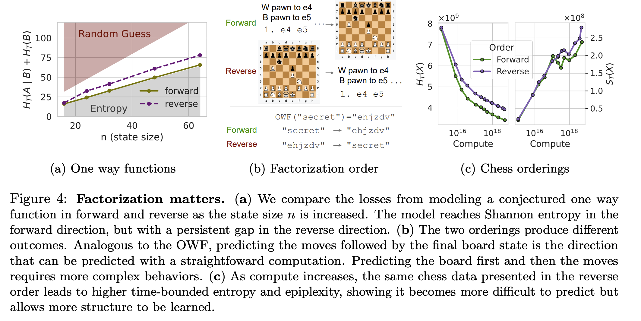
• (a): forward direction of one-way function is easy to learn and approaches the Shannon entropy, the reverse direction doesn’t
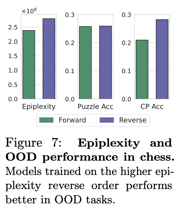
• (b, c): going from board position to chess moves is harder, but provides more structure / epiplexity to learn for larger compute regimes

5.3 The cap on what maximum likelihood modeling can learn is just to match the data generating process

5.3.1 “Induction” (not in the math sense, or in the induction heads sense)

Intuition for why this should be wrong: guessing the answer to a murder mystery (“induction”), which the model is trained for, is harder than being the author and knowing the murderer and just writing the murder mystery to be consistent with it

They mimic this by taking some bitstring $Z$, and applying some function $f$ to it, and also some masking $m(Z)$ to it, and only giving $(m(Z), f(Z))$ as the training pairs, so the model has to induct what the original $Z$ is from $m(Z)$.

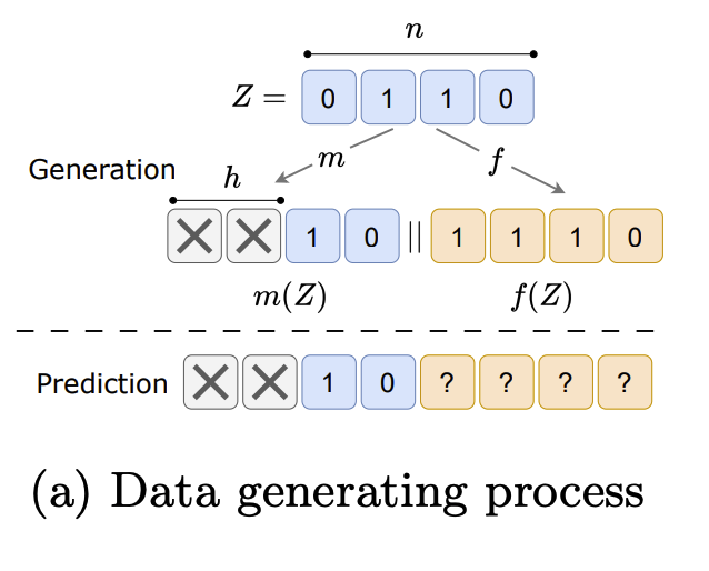
Case 1: $f(Z)$ is a one-way function. Then the model just learns to brute force all $2^h$ missing bit combos for $Z$, and the irreducible loss is hence $h$. The epiplexity still grows as $h$ grows because transformers aren’t perfect Turing machines and hence can’t write for loops: the program size to iterate over $2^h$ combos grows as $h$ grows

Case 2: $f(Z)$ is a Markov chain with $h / 8$ of states not having known transitions. Then at $h=0$ it just learns to deterministically apply the rules, and at $h=8$ it learns to just use past empirics on the transitions, but at $0 < h < 8$ it has to combine both which leads to higher epiplexity

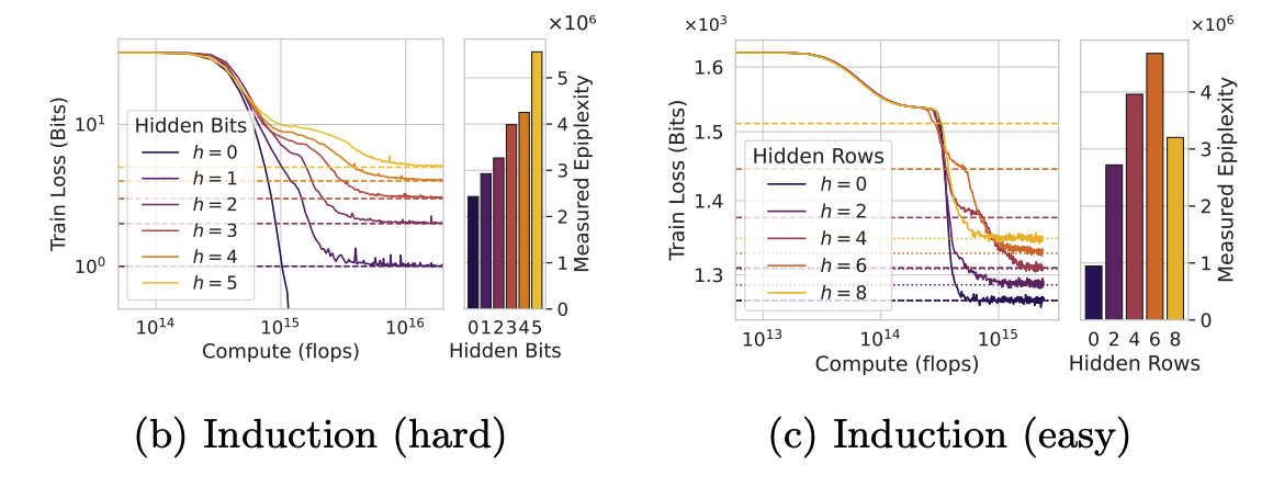
So the point being that epiplexity captures this kind of induction reasoning

5.3.2 “Emergent”

Conway’s game of life, if you have the compute (like a looped transformer) you can just brute force the computation, if not you need to think about gliders and what happens when they collide to predict the future and you learn more structure, more epiplexity.

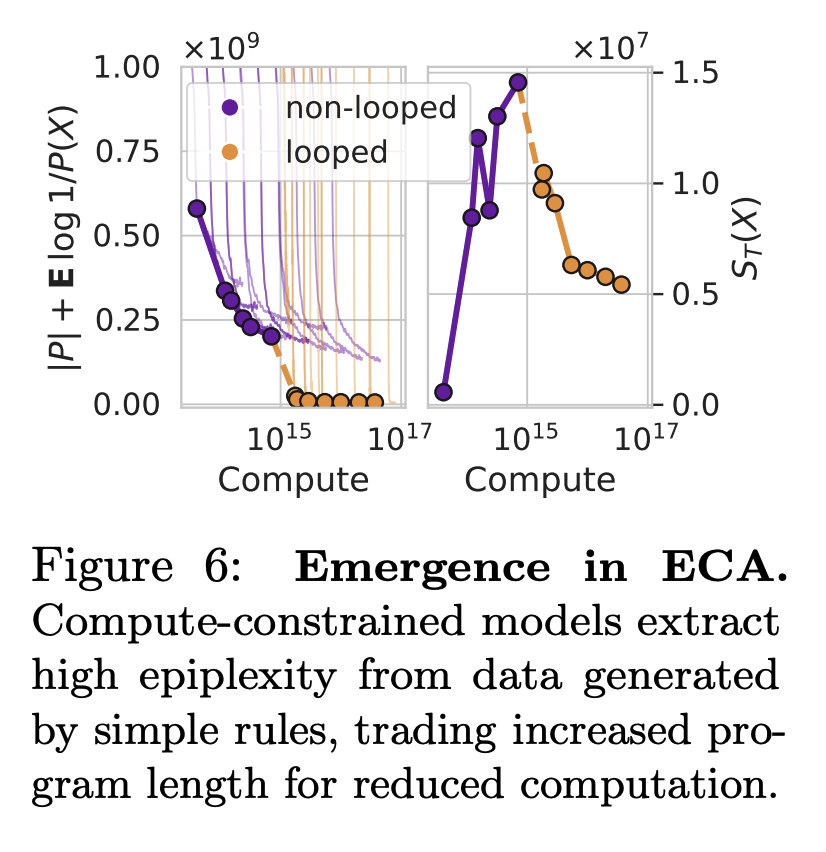
• at some level of compute, the brute force approach becomes possible and there’s less epiplexity because it just quickly learns that

Section 6: higher epiplexity predicts better OOD generalization

Intuition: epiplexity = learned general structure, irreducible loss is domain specific.

Of the two chess orderings from 5.2, the one with higher epiplexity generalizes better to predicting centipawn accuracy (more OOD than predict the next move puzzles)

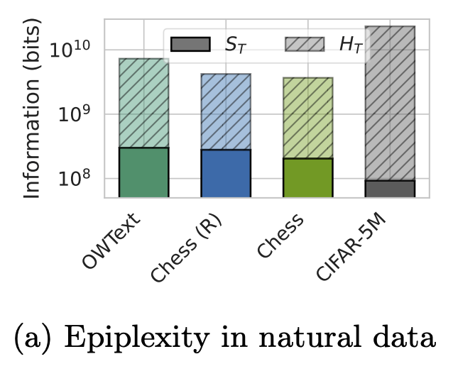
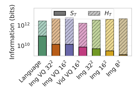
• They show that language pretraining data has a higher epiplexity content than image pretraining data

Assuming scaling laws, you can solve for the maximum epiplexity of a data set under infinite compute: it turns out to be when you train on exactly one epoch of the full data (past that, you’re not decreasing the entropy by enough to justify the increase in program length).

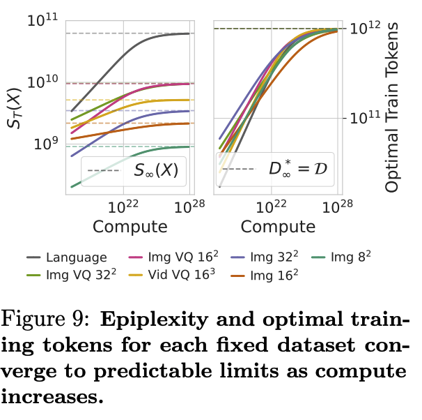
This once again corroborates that language has higher epiplexity than vision