mHC: Manifold-Constrained Hyper-Connections

Motivation: From one layer of activations to the next, what are different designs you could choose for the backbone? If you remember the mathematical transformer paper, you should still be thinking of layers as operations on this backbone, but now sometimes we apply a transformation to the backbone itself

From left to right: residual connection (literally just have a residual stream of the original input the whole way through), hyperconnections, and finally deepseek’s things manifold constrained hyper connections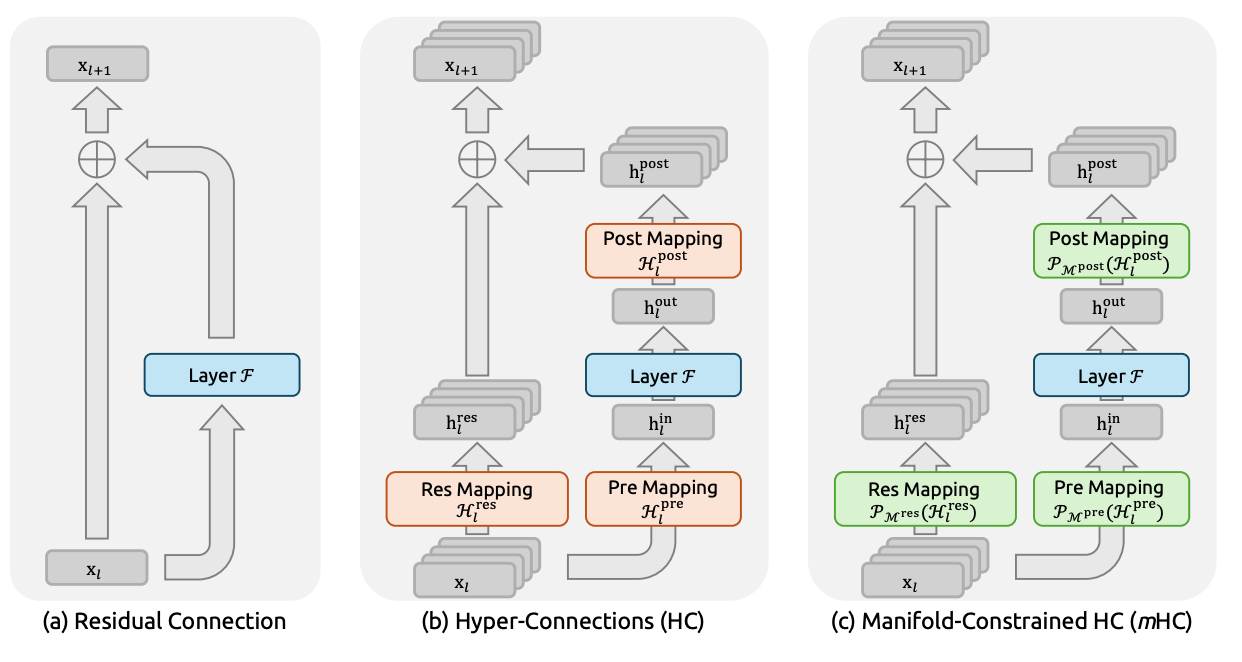

1. residual connections: a review. Why do we want these?
   1. It allows you to “skip layers.” The default operation of a layer is to do nothing, which is nice by Occam’s razor. The loss landscape becomes a lot nicer — no vanishing gradients, and not every layer is multiplied together in every added together term in the gradient chain rule.
2. Why hyper connections (papers from 2024)?
   1. It turns out that the residual stream is doing a lot of work. Bottleneck superposition says that there are way more than C dimensions of meaning being stored in the C dimensional residual stream. Wouldn’t it be nice if we had n _ C dimensions instead? But then if we made d_model = n _ C dimensions, we would have n _ C dimensions for all of our layer operations, like attention and the FFN would be on n _ C dimensional vectors, which is pretty bad for FLOPs. We’d like to keep our layer computation themselves C dimensional.
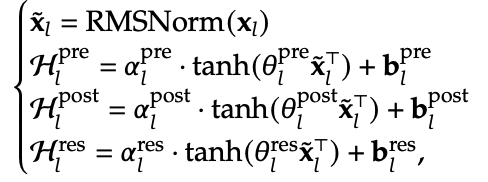
   2. Enter hyper-connections: we make the residual stream an n x C matrix, and then we simply have the matrices H^pre compress this down to a C dimensional vector before a layer, and then H^post project this back up to n x C after a layer. These mappings have very particular functional forms that I don’t have good intuition for. I’m just aware that they have some component that depends on the input, which is interesting — you’re not learning a static projection.
      1. The matrix multiplication from an n x C to a 1 x C is only order nC FLOPS which is cheap af.
   3. 
   4. What’s also super cheap is storing the weight matrices to do these operations. Like n = 4 here, so these are at most O(C) which is basically costless, since in FFN for instance, you have weights O(C^2).
   5. What is this H^res? Well, turns out we don’t want the n residual channels to just be fully independent from each other, for the same reason that Independent component analysis (ICA) is not really a thing, and PCA is actually good. So H^res exists to mix together the residual streams. More on this later in mHC
3. What’s the problem with hyper connectors?
   1. Now, if you look at the path along the backbone from the input to the output, the input x gets multiplied by a ton of pretty arbitrary matrices. So this is kind of bad because we lose most of the nice benefits from residual connections. Like now, we could easily have exploding gradients from these matrix multiplications.
   2. 
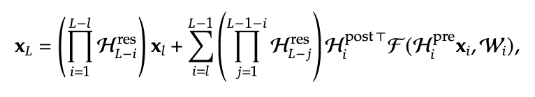
   3. the first term is what’s making us sad, because that’s not the identity
4. mHC
   1. instead of letting H^res be an arbitrary matrix, we project it into a doubly stochastic matrix, i.e. a matrix which has rows and columns summing to 1. These matrices have three nice properties:
      1. they have bounded spectral norm, so they don’t lead to exploding gradient
      2. they’re closed under multiplication. This makes it so that the first term is also a doubly stochastic matrix
      3. they can be interpreted as the convex hull of the set of permutation matrices. So this operation on the residual stream is really just a convex combination of “mixes” of the residual stream
   2. And now you see that we’ve solved the optimizing landscape problem by i, and ii and iii make it so that our Occam’s razor now is that the default operation should be to mix around the n residual streams, which seems pretty fair

Great, so what’s the problem now? well the problem is that you now have a ton of nC sized activations. So you have to do a ton of work to make sure that you’re not intensely memory-bottlenecked.

• The one trick that I understood was that they saved only like every X’th layer’s residual activation (size nC) during the forward pass, preferring to recompute them during the backward pass. This is standard. But what they did that I don’t think is standard is they saved the output (C dimensional) of every layer F (from the original picture). Because those are smaller so they take less memory, and they’re also the most computationally expensive parts of the forward pass, so you get to save a lot of compute on the backward pass.
• a ton of kernel fusion, which is basically GPU coding that does the order of operations in an equivalent way that avoid a lot of the communication cost
• some pipelined parallelism nonsense

How were their results? Well their actual performance improvement was pretty marginal.

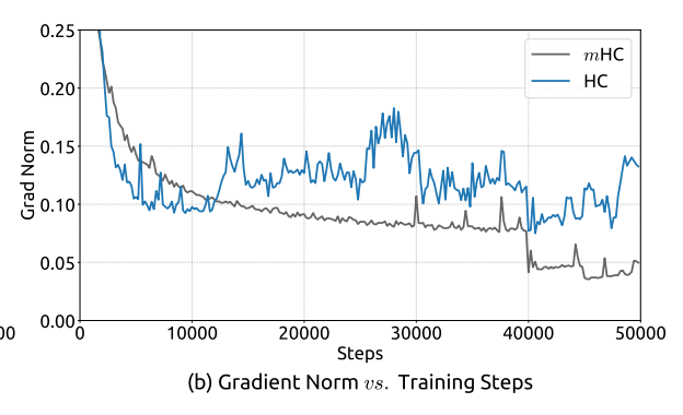This is the most impressive one to me. They have way stabler gradients during training, even compared to the residual connection baseline.

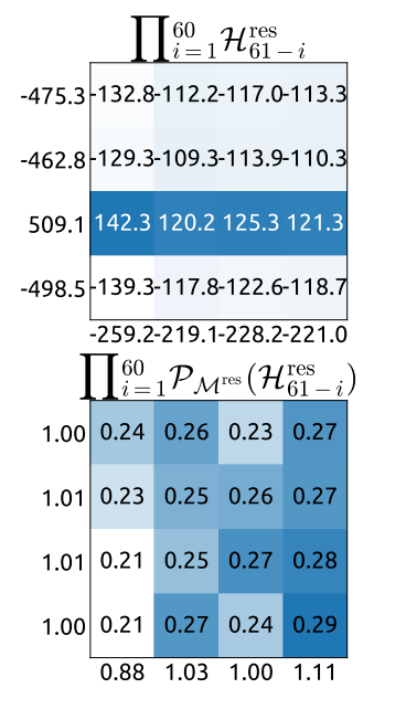Seems like their mixing (bottom) is also much better than the standard hyperconnection mixing (top)