What are Diffusion Models?

many many different sources cited this blog post. From what I can tell, it is actually quite comprehensive for the evolution of diffusion pre like 2024

Forward diffusion process

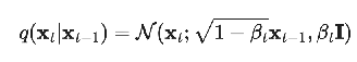can jump many steps forward at once 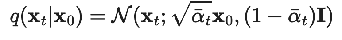reframed as the key nice property, a relationship between x_0, x_t, and epsilon_t

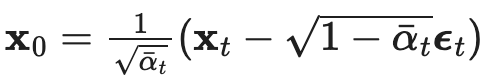
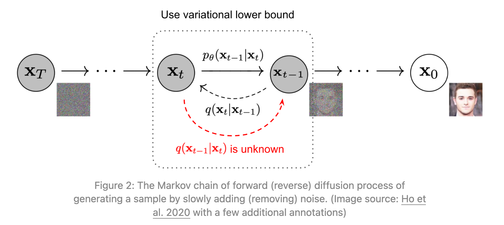
reverse process intuition

Goal is to approximate q(x_{t-1}

x_t). Can’t calculate that directly since it involves an integral over the entire dataset, so do that using a neural network: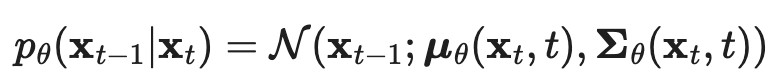

But how are we going to train this neural network, if we can’t accurately calculate q(x_{t-1}

x_t)?

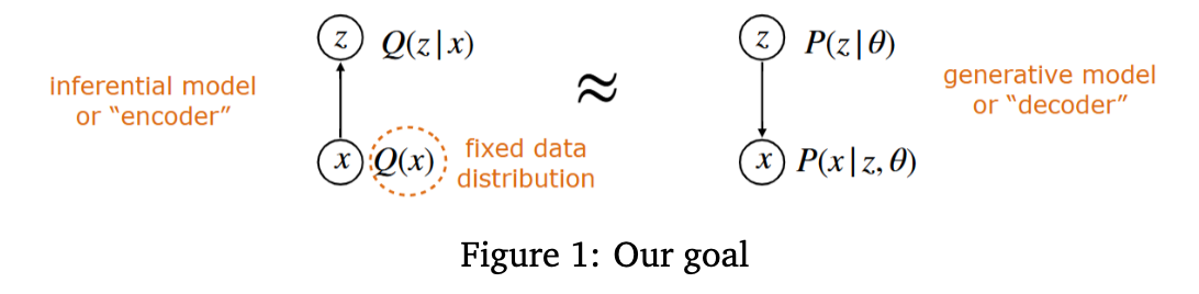
You can interpret what we’re doing with the forward and backwards process as the standard VAE architecture, with time 0 as the observed, and times 1:T as the latent.

Then the ELBO Loss includes terms that look like KL(q(x_{t-1}

x_t, x_0)

p_theta(x_{t-1}

x_t) ), i.e. we’ll instead be able to train the reverse process predictor neural net against the conditional reverse process knowing x_0. And it won’t be biased because when we minimize the expectation of this KL over x_0 and x_t drawn from the forward process, you actually get p_theta(x_{t-1}

x_t) to equal to the marginal q(x_{t-1}

x_t).

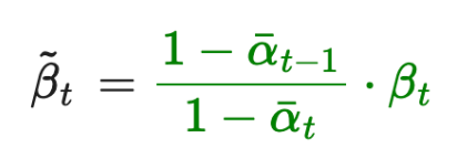
Deriving q(x_{t-1} | x_t, x_0)

by Bayes Rule 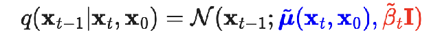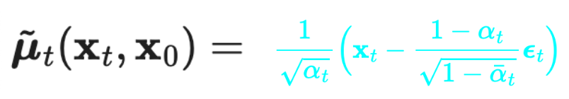(where we’ve expressed the mean in terms of the noise epsilon_t, back from the forward process)

A brief review of VAEs and ELBO from 6.7900

We would like to train the network by just maximizing the log likelihood log P_theta (x). For now, just assume that we’re working with a single data point x. You can take an expectation over all the x’s in the dataset later

The problem is that it’s hard to instantiate P_theta(x), because we only really have nice forms for P_theta(x

z). The way we get around this is by maximizing the ELBO loss wrt theta instead

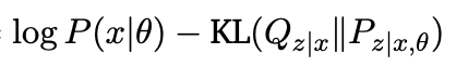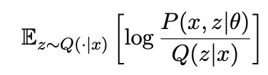
ELBO = = Note that for a fixed Q(z | x), ELBO is maximized when we optimize theta so that P_theta(z | x) exactly matches Q(z | x). The EM algorithm now looks like

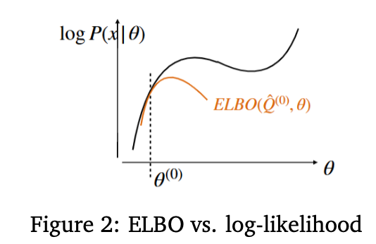
maximize ELBO wrt theta, with Q(z x) fixed. This pushes the ELBO score up

redefine ELBO by setting Q(z

x) := P_theta(z

x). This also pushes the ELBO score up because it makes the KL loss smaller. And what we have at this point is exactly the log P_theta(x), which means that we’ve managed to push that up. Rinse and repeat this process.

At a high level, EM algorithm is just fixing the latent prediction distribution, then using that to optimize the parameters, and then using the resulting parameters to improve the latent prediction, and repeating. ELBO is just rigorizing the fact that this works to actually increase the log likelihood of the data.

Applying VAE ELBO loss to diffusion models

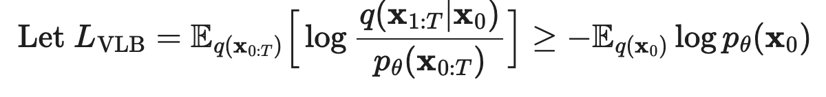
Here, the actual data distribution is x_0, and the latent is x_{1:T}. So fixing an x_0, we would get that the (negative) ELBO is

E_{Q(x_{1:T}

x_0} [ log Q(x_{1:T}

x_0) / P_theta(x_0, x_{1:T}) ] >= - log p_theta(x_0)

And then taking expectation over both sides of x_0 (the dataset distribution), we get the equation from the blogpost

Now using the structure of the forward process being a markov chain, and doing a bunch of logarithm rearrangements, we get that this ELBO loss is equal to 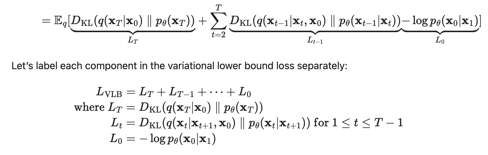This is now trainable, since L_T is constant, L_0 we do something about which I’m not totally sure, and L_t’s are KL’s of gaussians which has a closed form. Let’s dig a little deeper into that L_t term.

Note that instead of predicting the mean of x_{t-1}, we can just aim to predict the noise epsilon_t that was added to get from x_0 to x_t, since we previously derived an expression for the mean using this noise. So we reparameterize from µ_theta(x_t, t) to epsilon_theta(x_t, t), and then we expand out the closed form formula for the L_t KL loss, getting us to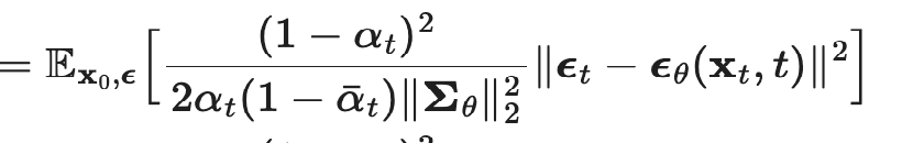

But then empirically, training this just works better (ignoring the weight term at the beginning) 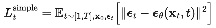Which results in the following algorithm

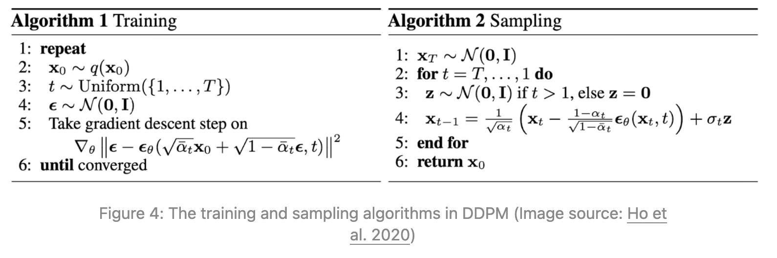
I think the sigma_t is just the coefficient of the covariance that we derived when we were doing the p(x_{t-1} x_t, x_0) calculation

Connection to score-based methods

ignoring lilian weng’s explanation for this part because it’s remarkably useless see pages 16-17 of https://arxiv.org/pdf/2208.11970 instead

Basically , remember how we had the nice relationship between x_t, x_0, and epsilon_t? Well since x_t | x_0 is a Gaussian, we can actually apply Tweedie’s Formula to get a relationship between x_t, x_0, and the score function: 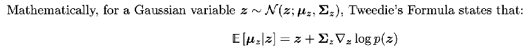so applying that to x_t | x_0, we get 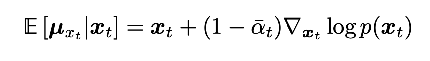plugging in that the mean is sqrt(alpha bar_t x_0), we get the relationship 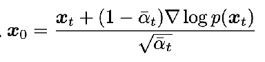We can plug in x_t in terms of x_0 and epsilon_t from the nice property to get a key relation between just the score and epsilon_t:

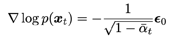
just a scaled (time-dependent scaling factor) version of the source noise
intuitively, the score function measures direction to maximize log probability
moving in the opposite direction of source noise “denoises” the image and is the best update to increase log probability

So we have three equivalent parameterizations of the training:

predicting the mean of x_{t-1} directly given x_t, t
predicting the source noise epsilon_t given x_t, t
predicting the score function s(x_t, t) given x_t, t

Conditional Diffusion

Classifier-Guided Basically now, we want to generate images conditioned on being from a certain class in the dataset. How can we do that, assuming we have a good classifier for the class?

Answer: instead of optimizing for the score function of q(x), we optimize for the score function of q(x, y) and plug in the class for y. 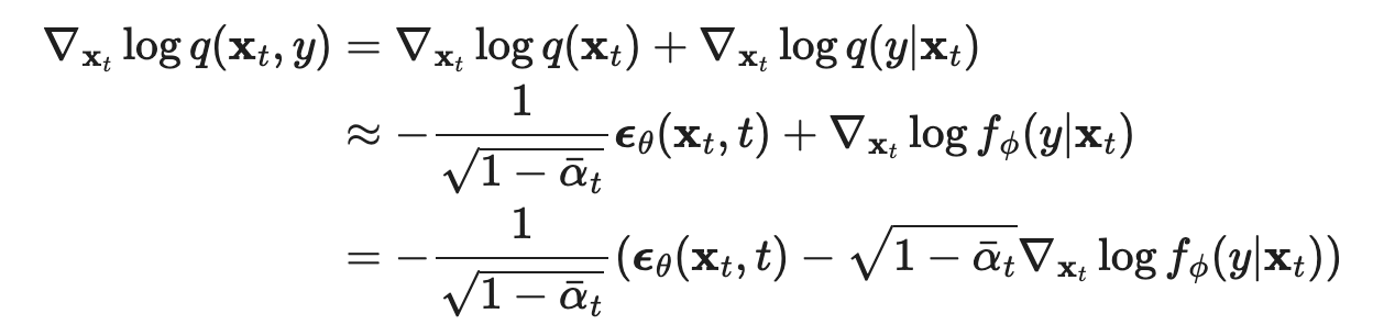Using the connection to score based methods, this implies using this updated noise for the denoising process instead. Classifier-Free What if there was a way to train the diffusion model itself to be able to estimate that gradient log f_phi(y | x_t) term? Turns out there is: learn one network that learns to predict both unconditional noise e_theta(x_t, t), as well as conditional noise e_theta(x_t, t, y), by giving it training data of both types.

Then we can write the gradient term we need as 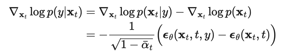So we can plug that back into the conditional noise equation to get the right effective conditional denoising amount

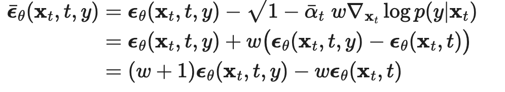
Speeding up diffusion models (because they are SLOW)

DDIM (denoising diffusion implicit model)

Earlier, we did an exact calculation for q(x_{t-1} | x_t, x_0). This time, let’s write the reverse update step as 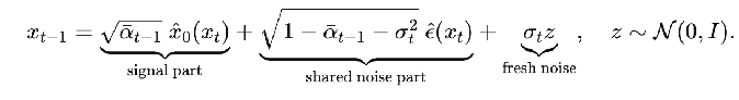i.e. reparameterize into the deterministic part and the new randomness added in this step.

And then for DDIM, you set sigma_t = 0, so the whole reverse process is now deterministic. This corresponds to a different forward process (you’re no longer adding new fresh independent noise at each step), but the marginals still agree, so it’s not actually a problem that we don’t have randomness. Why is this useful? On its own, it allows us to do some step skipping, but it helps with other techniques, such as :

Progressive distillation Given a teacher deterministic sampling model, distill it into a student model which basically learns to do two denoising steps at once (recall that the reverse process is basically just learning what x_{t-1} | x_t was), thus halving the number of steps. Repeat this until you get to your desired number of steps in the reverse process.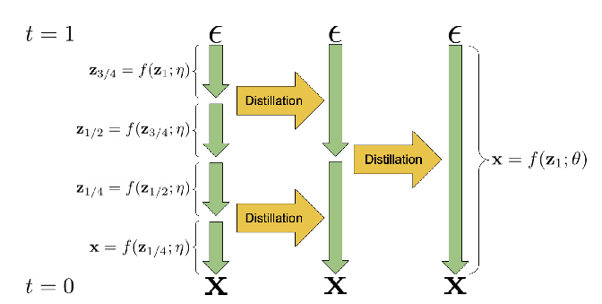

Consistency Models 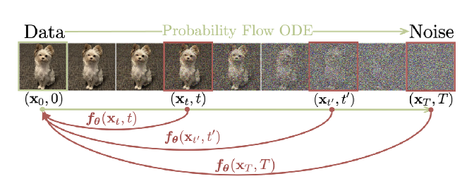Main idea is to learn a model that can predict in one-shot the original image from any point of noise

You can train one of these by distilling an existing diffusion model, or by training from scratch.

Distilling existing model: training objective is basically to take one step of an ODE solver on the current timestep to get the next timestep, and then minimize the distance between the original predicted image for these two adjacent timesteps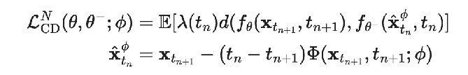

theta- : the target we’re matching to is a exponential weighted moving average (slower, smoother) version of the network

Consistency Training is their term for training from scratch

Instead of using one step of the ODE, they use one random gaussian draw and add noise scaled with adjacent timesteps’ scales

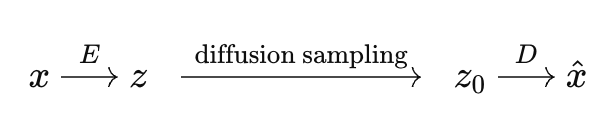
Latent diffusion models

Main idea is that denoising entire images, with all the pixels in them, is unnecessarily slow. We can compress the images into a smaller latent space using an autoencoder, and then run reverse diffusion on the latent, and then decompress it back into the full image

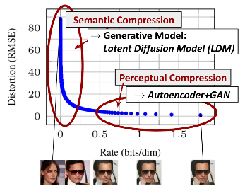the main gain is that the autoencoder is doing the perceptual compression, while the diffusion model is doing the semantic compression

Scaling up generation resolution and quality

Approach #1: Ho et al.

Idea is to use a cascade of diffusion models, where the first diffusion model predicts a low resolution image, and then later diffusion models are conditional diffusion: conditioned on the previous lower dim image, they reverse diffuse the next higher resolution image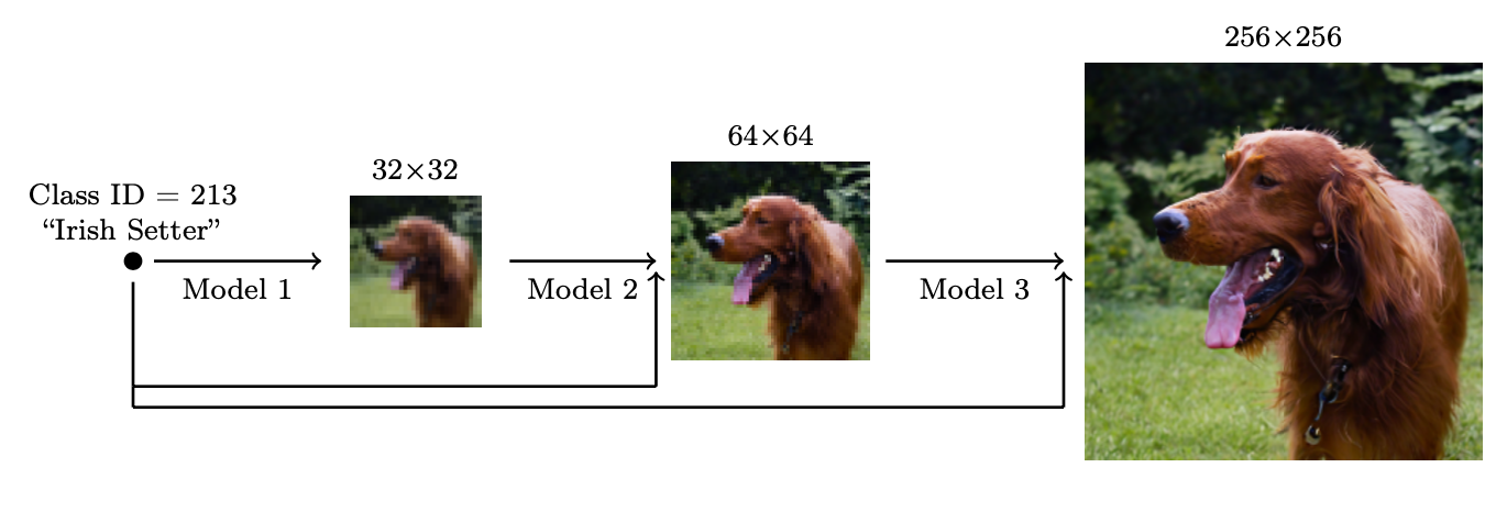

one of the key problems is that when you’re training, you want to give the model exposure bias to “bad” conditioning data to avoid having cascading error (since now the models are used to the inputs being bad already), which you do by adding some noise to the conditioned inputs (which can also be done by just stopping the reverse diffusion process early)

add gaussian noise for low res, gaussian blur for high res

unCLIP also has the upsampling reverse diffusers, but their main innovation is using CLIP on the input text, which generates an embedding (the processed version of this embedding is what they call the prior) that we then do conditional diffusion on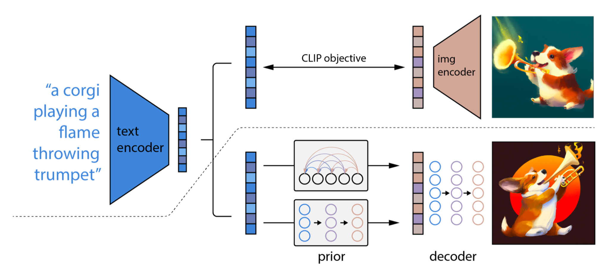

Imagen

basically polishing the ideas from before: use T5-XXL instead of CLIP as the text encoder, still use cascaded diffusion, tweak the guidance-based conditional diffusion to make sure that the x_0’s stay within distribution, and make the architecture a little more efficient

Model Architectures

U-Nets are lowkey dying so not too much need to look too deeply into them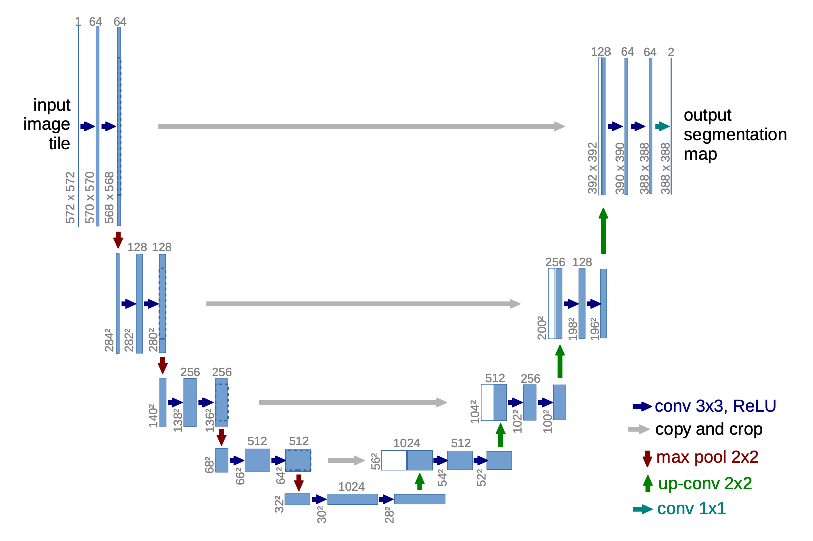

Diffusion Transformers

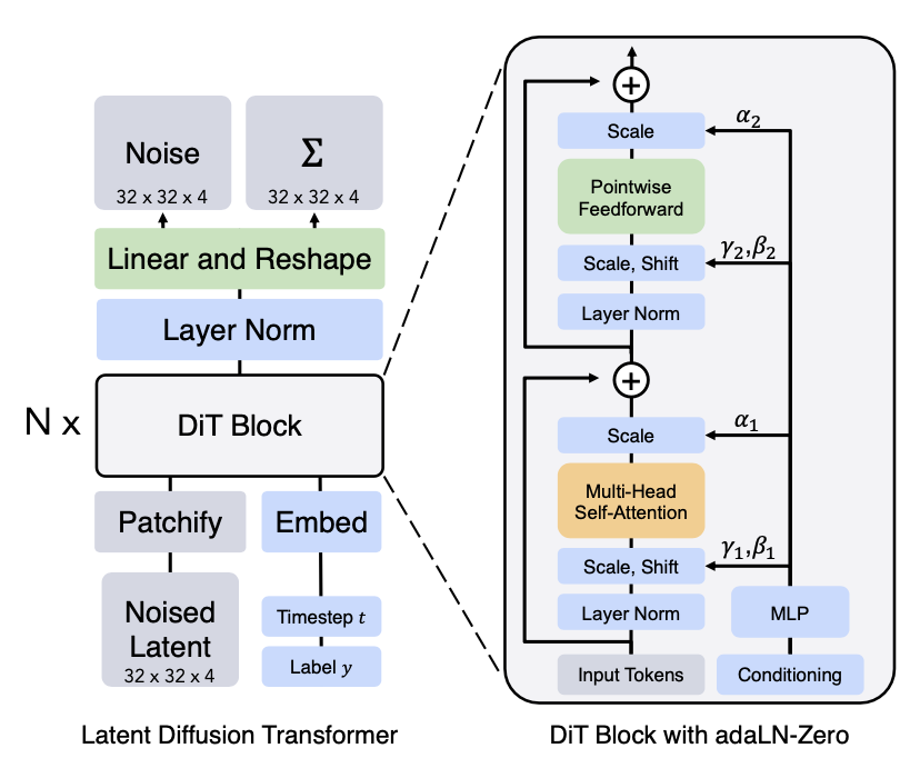
patchify is literally just split the noised latent input into patches of size p and put them into a sequence
adaLN-Zero just refers to the gamma_1, beta_1 etc way of encoding the label y as part of conditional generation. This was just empirically the best method they came up with